Reweighting

Ostap offers set of utlities to reweight the distributions. Typical use-case is

one has set of data distributions
and simulation does not describe these distributions well, and one needs to reweight simulation to describe all distributions

It is relatively easy procedure in Ostap, however it requires some code writing.

Data and simulated distributions

First, one needs to specify data distributions. It can be done in form of 1D,2D and 3D histograms, or as 1,2, or 3-argument functions or even all these techniques could be used together. It is important that these data distributions should be strickly positive for the corresponding range of variables. E.g. in case of histograms, there should be no empty or negative bin content.

hdata_x = ROOT.TH1D ( ... )               ## e.g. use the histogram 
hdata_x = lambda x :  math.exp (-x/10 ) ) ## or use a function 
...
hdata_y = ...

Second, for each data distribution one needs to prebook the corresponding template histogram that will be filled from simulated sample. This template histogram should have the same dimensionality (1,2,3) and the corresponidg data distribtion. If data distribution is specified in a form of historgam, the edges of prebooked template histogram should correspond to the edges of data distribution, but there is no requirements for binning. Binning could be arbtrary, provided that there are no empty bins.

hmc_x = ROOT.TH1D ( ... )
hmc_y = ....

Iterations

Third, one needs to create empty database where the iterative weights are stored:

import Ostap.ZipShelve as DBASE 
dbname = 'weights.db'
with DBASE.open( dbname ,'c') as db : 
     pass

Since Reweighting is essentially iterative procedure, we need to define some maximal number of iterations

iter_max =   10 
for iter in range(iter_max) : 
   ...

Weighter object

And for each iteration we need to create weighting object, that reads the current weights from database weight.db

from Ostap.Reweighting import Weight  
weightings = [
    ##         accessor function    address indatabase    
    Weight.Var ( lambda s : s.x  , 'x-reweight'  ) ,
    ...  
]    
weighter   = Weight ( dbname , weightings )

What is it?Click to expand

The accessor function is used to get the variable from simulated sample. E.g. in this form, TTree/TChain/RooDataSet/RooArgSet can be used as source of simulated data. but it could be also e.g. some table, numpy array or any other storage. In this case the accessor function needs to be modified accordingly. The second parameter specify the location in (newly created empty) database, where the current weights are to be taked from. Since the newly created database is empty, for the first iteration all weights are trivial and equal to 1:

mc_tree =  ...
for i in range(100): 
  mc_tree.GetEntry(i) 
  print ' weight for event %d is %s' % ( i , weighted (  mc_tree ) )

Weighted simulated sample

As the next step one needs to prepare simulated dataset, RooDataSet, that

contains all varables for reweighting
the current values of weights, provided by weighter-object above

There are many ways to achive this. E.g. one can use SelectorWithVars-utility to decode data from input TTree/TChain into RooDataSet:

from Ostap.Selectors   import SelectorWithVars, Variable  
## variables to be used in MC-dataset 
variables  = [
   Variable ( 'x'      , 'x-var'  , 0  , 20 , lambda s : s.x ) ,  
   ...
   Variable ( 'weight' , 'weight' , accessor = weighter       )  
   ]
## create new "weighted" mcdataset
selector = SelectorWithVars (
   variables ,
   '0<x && x<20 && 0<y && y<20'
   )
## process 
mc_tree.process ( selector )
mcds = selector.data      ## newly created simulated dataset
print mcds

Calculate the updated weights and store them in database

At the next step we calculate the updated weights and store them in database

from Ostap.Reweighting import makeWeights,  WeightingPlot  
plots  = [
  ##             what      how        where          data      simulated-template 
  WeightingPlot ( 'x'   , 'weight' , 'x-reweight'  , hdata_x , hmc_x       ) ,  
  ...
  ]
## calculate updated weights and store them in database 
more = makeWeights ( mcds , plots , dbname , delta = 0.01 ) ## <-- HERE

The object WeightingPlot defines the rule to fill simulated histogram from simulated dataset and associated the filled simulated histogram with data distribution. The actual correction to the weights is calculated according to the rule w = dd / mcd, where dd is a density for the data distribution and mcd is a density for simulated distribution. The weights w are calculated for each entry in array plots, they are properly normalized and stored in database dbname to be used for the next iteration. The function makeWeights also print the statistic of normalized weights:

# Ostap.Reweighting         INFO    Reweighting:           ``x-reweight'': mean/(min,max):        (1.00+-0.00)/(0.985,1.012) RMS:(0.74+-0.00)[%]

The last entries in this row summarize the statistics of corrections to the current weight. In this example, the mean correction is 1.00, the minimal correction is 0.985, the maximal correction is 1.012 and rms for corrections is 0.74\%. In tihs example one sees that for this paricualr iteration th ecorrections are rather small, and probably one can stop iterations. Two parameters delta and minmax of makeWeights function allows to automatized th emakinnng the decison. If calculated rms for all corrections is less than specified delta parameter and for each correction minnmax-difference deos not exceeed the specified minmax-parameter (the default value is 0.05), function return False (meaning no more iterations are needed), otherwise it returns True. And using this hint one can stop iterations or go further:

if not more and iter > 2 :
    print  'No more iteratinos  are needed!'
    break

Compare data and simulated distributions for each iteration (optional)

In practice it is useful (and adviseable) to compare the data and simulated distributions at each iteration to hjave better control over the iteration process. One can make this comparion using zillions of the ways, but for the most imnportant case in practice, where data distribution is specified in a form of histogram, there are some predefined utilities

## prepare simulated distribution with current weights:
mcds.project ( hmc_x , 'x' , 'weight' ) 

## compare the basic properties: mean, rms, skewness and kurtosis
hdata_x.cmp_prnt ( hmc_x , 'DATA' , 'MC' , 'DATA(x) vs MC(x)' )

## calculate the ``distance``:
dist = hdata_x.cmp_dist ( hmc_x , density = True )
print "DATA(x)-MC(x)  ``distance''        %s" % dist 

## calculate the 'orthogonality'
cost = hdata_x.cmp_cos  ( hmc_x , density = True )
print "DATA(x)-MC(x)  ``orthogonality'' %s" % cost 

## find the points of the maximal difference 
mn,mx = hdata_x.cmp_minmax ( hmc_x   , diff = lambda a,b : a/b , density = True )
print "DATA*(x)/MC(x) ``min/max-distance''[%%] (%s)/(%s) at x=%.1f/%.1f" % (
        (100*mn[1]-100) , (100*mx[1]-100) , mn[0]  , mx[0] )

Using the result

from Ostap.Reweighting import Weight  
weightings = [
    ##         accessor function    address indatabase    
    Weight.Var ( lambda s : s.x  , 'x-reweight'  ) ,
    ...  
]    
weighter = Weight ( dbname , weightings )
mc_tree  =  ...
for i in range(100): 
  mc_tree.GetEntry(i) 
  print ' weight for event %d is %s' % ( i , weighted (  mc_tree ) )

Note that due to explicit specification of accessor function, reweighter can be customised to work with any type of input events/records. e/g/ assuem that event is a plain array, and x-variable corresponds to index 0:

from Ostap.Reweighting import Weight  
weightings = [
    ##         accessor function    address indatabase    
    Weight.Var ( lambda s : s[0]  , 'x-reweight'  ) ,
    ...  
]    
weighter = Weight ( dbname , weightings )
mc_tree  =  ...
for event in  events : 
  print ' weight for event %s is %s' % ( event , weighted ( event ) )

Abstract reweightingClick to expand

Abstract reweighting

Due to the freadom in choosing the accessor function, one can apply reweighting procedure to the absolutely abstract samples. E.g. consider the follwing case

data distribution : simple function
simulated sample : random number generator

As a result of reweighting procedure, we'll get reweighted simulated sample, that will be just a random number generator, that produces the weighted distribution according to the specified function. For this case, the code is very transparent and compact:

# =============================================================================
## 1)  ``DATA distribution''  - plain function
def data ( x ) :
    return 0.5 + math.sin ( x * math.pi )**2 
# =============================================================================
## 2) ``simulation template'' -  histogram template for simulated sample 
mc_hist = ROOT.TH1F ( 'hMC', '', 20 , 0 , 1  )
# =============================================================================
def mc_sample () :
    x = random.expovariate ( 1 )
    while x  > 1  : x -=1
    return x
# =============================================================================
## 3) create empty database with initial weights 
# =============================================================================
import Ostap.ZipShelve as DBASE
if os.path.exists ( dbname ) : os.remove ( dbname )
with DBASE.open( dbname ,'c') as db :

And then one starts iterations:

# ============================================================================
## 4) prepare reweigthing iterations
# ===========================================================================
from Ostap.Reweighting import Weight, makeWeights,  WeightingPlot
from Ostap.Selectors   import SelectorWithVars, Variable   
for iter in range ( 100 ) :    
    ##                                             accessor       address in DB    
    weighter   = Weight( dbname ,  ( Weight.Var ( lambda x : x , 'x-reweight'  ) , ) ) 

    ## create ``weighted'' simulated  dataset using the current weights
    selector = SelectorWithVars (
        selection  = '1<2' , ## fake one :-( to be removed soon 
        silence    = True  , 
        variables  = [ Variable ( 'x'      , 'x-var'  , 0  , 1  , lambda x : x ) ,  
                       Variable ( 'weight' , 'weight' , accessor = weighter    ) ] )    
    for  i in  range ( 1000000 ) :
        x = mc_sample () 
        selector ( x )
    mcds = selector.data 
    ##  update weights: the rule to create weighted simulated histogram
    plots = [ WeightingPlot ( 'x' , 'weight' , 'x-reweight' , data , mc_hist  ) ]    
    ## calculate the updated weights and add them into   database  
    more = makeWeights ( mcds , plots , dbname , delta = 0.01 )
    if not more and 2 <= iter : 
        logger.info ( 'No more iterations are needed #%d' % iter )
        break

The full example for abstract reweighting, is accessible here

The density distribution for the simulated sample for before the first (blue open squares) and after the last (filled red points) iterations are shown here, iterations3 while the comparison of the initial data distribution (red line) and the reweighted simulated sample (greed filled diamonods) are shown here. results3

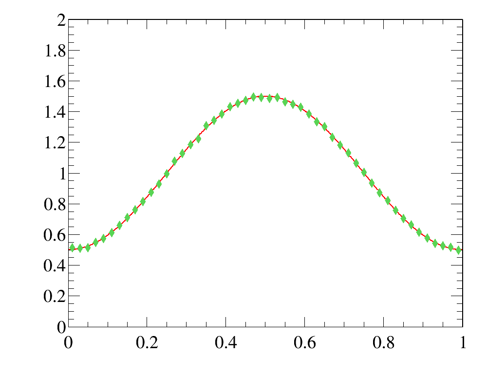
Why one needs iterations?Click to expand

Examples

Simple `1D`-reweighting

The example of simple 1D-reweighting can be inspected here, while the reweigthing result for the last iteration (blue open squares) are compared with data distribution (red filled circled) here: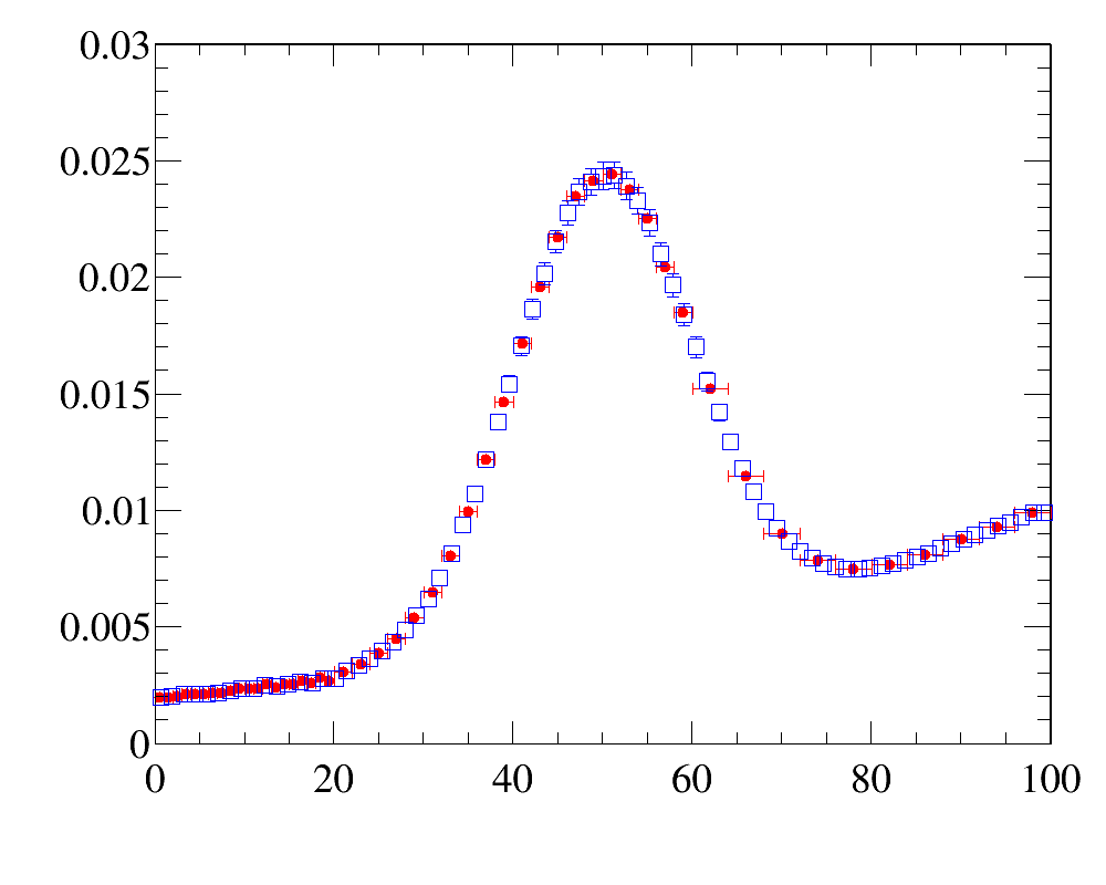

The example also illustrates how to use various histogram comparison functions to have better control over the iterative process

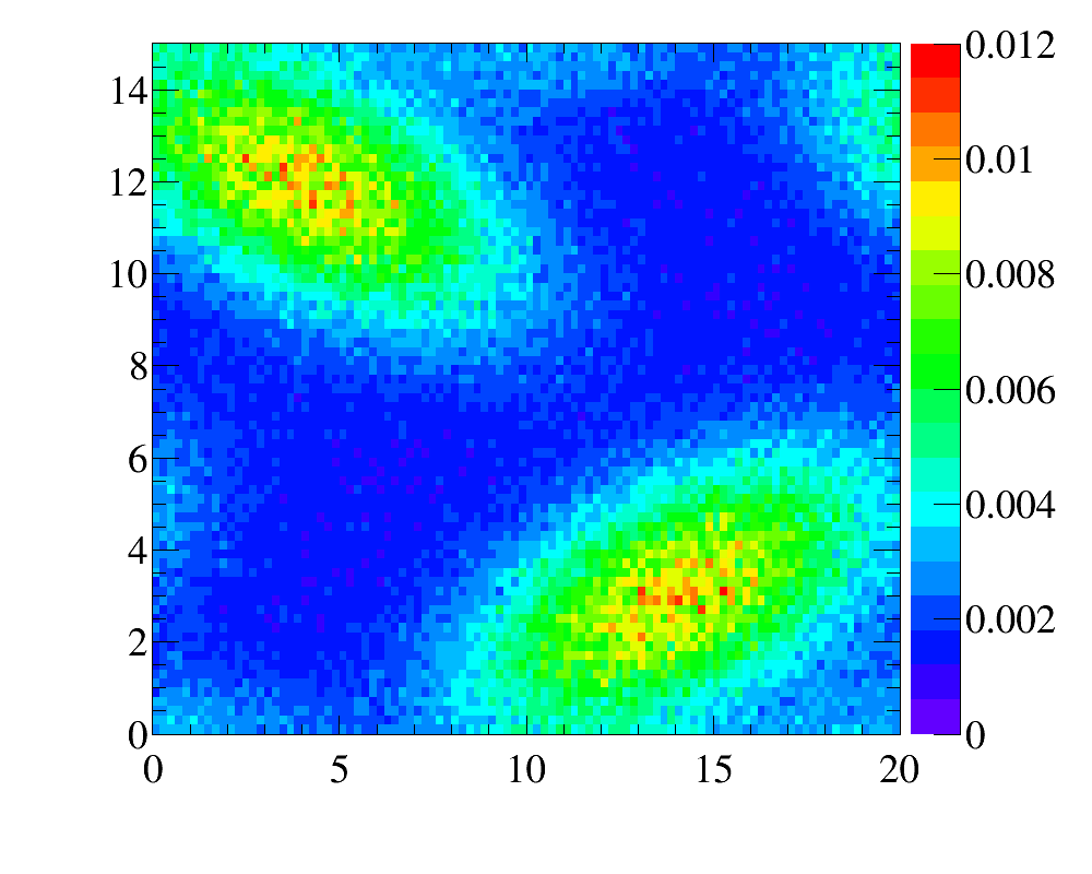
More complicated case of non-factorizeable `2D`-reweighting

The example of advanced 2D-reweighting can be inspected here. In this example we have three data distributions fro two variables 1 one-dimensional x-distribution with fine binninig 1 one-dimensional y-distribution with fine binninig 1 two-dimensional y:x-distribution with coarse binning

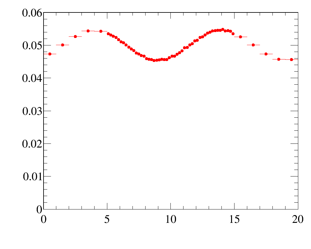
It reflects relatively frequent case of kinematic reweighting using the transverse momentum and rapidity. Typically one has enough events to make fine-binned one-dimensional reference distributions, but two-dimensional distributions can be obtained only with relatively coarse binning scheme.

Simulated sample is a simlpe 2D-uniform distribution. Note that the data distributions are non-factorizeable, and simple 1D-reweightings here is not enought. In this example, for the first five iteration only 2D-reweighting y:x is applied, and then two 1D-reweighting x and y are added.

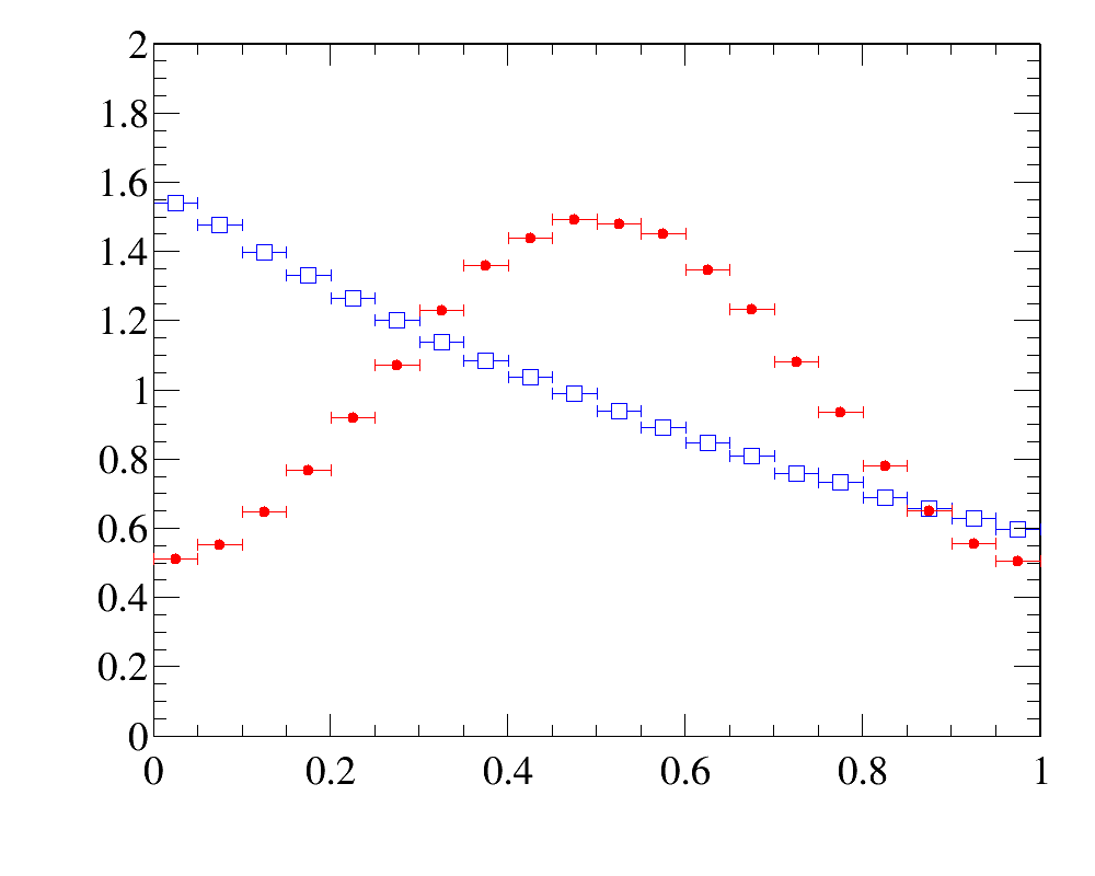
After the reweighting the simulated distributins are

for x-variable: data distribution (red filled circled) vs simulated sample (blue open squares)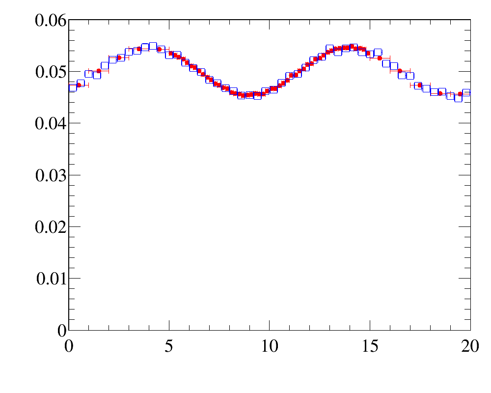
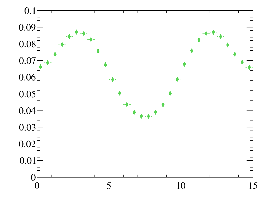
for y-variable: data distribution (green filled diamonds) vs simulated sample (orange filled swiss-crosses)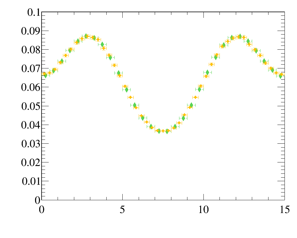
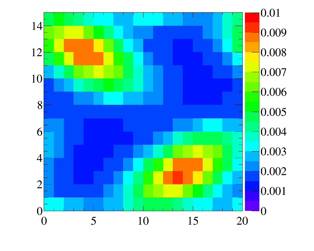
for y:x-variables

Reweighting

Reweighting

Data and simulated distributions

Iterations

Weighter object

What is it?Click to expand

Weighted simulated sample

Calculate the updated weights and store them in database

Compare data and simulated distributions for each iteration (optional)

Using the result

Abstract reweightingClick to expand

Abstract reweighting

Why one needs iterations?Click to expand

Examples

Simple `1D`-reweighting

More complicated case of non-factorizeable `2D`-reweighting

results matching ""

No results matching ""

Reweighting

Data and simulated distributions

Iterations

Weighter object

What is it?Click to expand

Weighted simulated sample

Calculate the updated weights and store them in database

Compare data and simulated distributions for each iteration (optional)

Using the result

Abstract reweightingClick to expand

Abstract reweighting

Why one needs iterations?Click to expand

Examples

Simple 1D-reweighting

More complicated case of non-factorizeable 2D-reweighting

results matching ""

No results matching ""

Simple `1D`-reweighting

More complicated case of non-factorizeable `2D`-reweighting