The LHCb data flow
Learning Objectives
Understand the LHCb data flow
Learn the key concepts on the stripping
The Large Hadron Collider provides proton-proton collisions to LHCb 40 million times a second. This results in a huge amount of data. In fact, if we were to store all the data coming in to LHCb, we would be recording ~ 1 TB every second.
That’s too much data for us to be able to keep all of it, the price of storage is just too high, so instead we need to filter the data and try to keep only the events which contain something interesting. This raises its own problems:
How do we filter and process the recorded data quickly and accurately?
How do we manage all the complex tasks required to work with collision data?
How do we organize all the data of a single bunch crossing in a flexible way?
How do we configure our software flexibly without having to recompile it?
Can you think of more?
These questions arise mostly due to two key points: the data must be processed very quickly because it’s arriving very quickly, and the data is complex so there’s a lot that can be done with it. In the last lesson we saw how many steps it took just to reconstruct a single decay, but there are thousands of possibilities that we might be interested in! Being able to perform such combinations in a flexible manner is then very important.
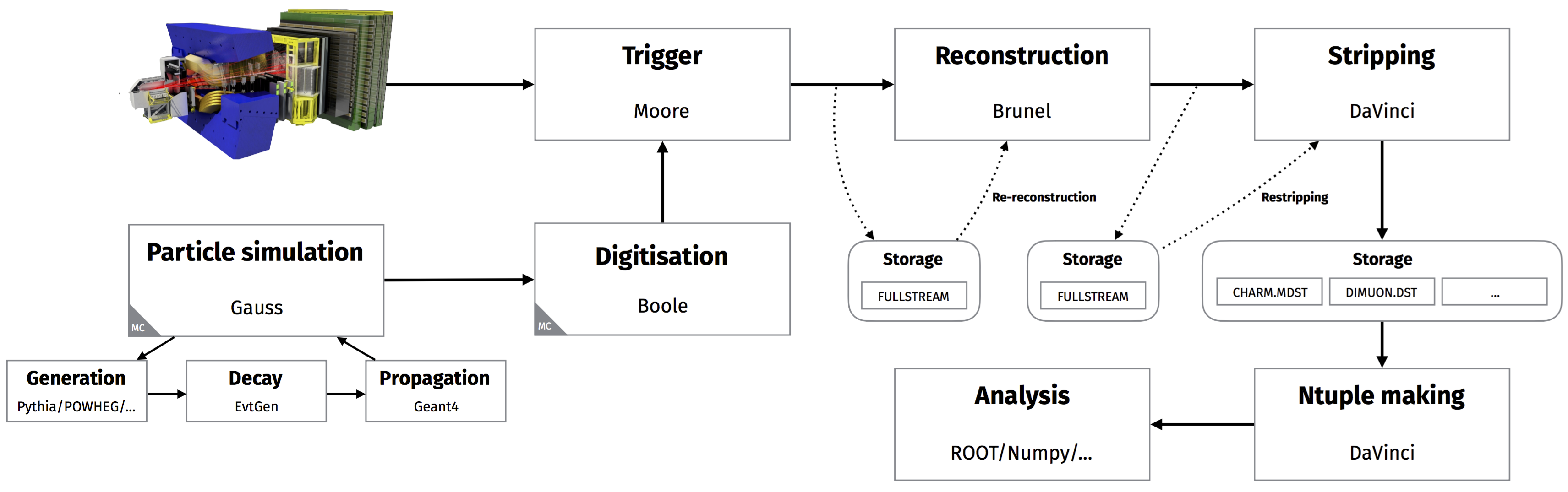
Collisions recorded by the LHCb detector go through a specific data flow designed to maximise the data-taking efficiency and data quality. This consists of several steps, each one being controlled by an ‘application’ that processes the data event-by-event, using the data from the previous step and creating the results ready for the next. These steps are as follows:
Data from the detector are filtered through the trigger, which consists of the L0, implemented in hardware, and the high level trigger (HLT), implemented in software. The application responsible for the software trigger is Moore, discussed in the trigger lesson in second-analysis-steps.
Triggered, raw data are reconstructed to transform the detector hits into objects such as tracks and clusters. This is done by the Brunel application. The objects are stored into an output file in a ‘DST’ format.
The reconstructed DST files are suitable for analysis, but they are not accessible to users due to computing restrictions. Data are filtered further through a set of selections called the stripping, controlled by the DaVinci application which write out data either in the DST or ‘µDST’ (micro-DST) format. To save disk space and to speed up access for analysts, the output files are grouped into streams which contain similar selections. By grouping all of the fully hadronic charm selections together, for example, analysts interested in that type of physics don’t waste time running over the output of the dimuon selections.
The output format
A DST file is a ROOT file which contains the full event information, such as reconstructed objects and raw data. Each event typically takes around 150kB of disk space in the DST format. The µDST format was designed to save space by storing only the information concerning the build candidates (that is, the objects used to construct particle decays like tracks); the raw event, which takes around 50kB per event, is discarded.
The overview of most important file formats used in LHCb can be found here.
Users can run their own analysis tools to extract variables for their analysis with the DaVinci application. The processing is slightly different between DST and µDST, since some calculations need the other tracks in the event (not only the signal), which are not available in the latter format.
We also produced lots of simulated events, often called Monte Carlo data, and this is processed in a very similar way to real data. This similarity is very beneficial, as the simulated data is subject to the same deficiencies as in the processing of real data. There are two simulation steps which replace the proton-proton collisions and the detector response:
The simulation of proton-proton collisions, and the hadronisation and decay of the resulting particles, are ultimately controlled by the Gauss application. Gauss is responsible for calling the various Monte Carlo generators that are supported such as Pythia (the default in LHCb) and POWHEG, and for controlling EvtGen and Geant4. EvtGen is used to describe the decays of simulated particles, whilst Geant4 is used to simulate the propagation and interaction of particles through and with the detector.
The simulated hits made in the virtual detector are converted to signals that mimic the real detector by the Boole application. The output of Boole is designed to closely match the output of the real detector, and so the simulated data can then be passed through the usual data processing chain described above, beginning with the trigger.
So, the data flow and the associated applications look like this:
Knowing this flow is essential in selecting your data! Different application versions can produce very different physics, so it’s very useful to know how each application has manipulated the data you want to use.
Why are there multiple applications?
It’s often simpler to create and visualise a single, monolithic program that does everything, but that’s not how the data flow is set up in LHCb. Why not? What are the advantages of splitting up the software per task? What are the disadvantages?
With the exception of a few specific studies, it is only the DaVinci application that is run by users, everything else is run ‘centrally’ either on the computing farm next to the detector or on the Grid.
The reconstruction, Brunel, is rarely performed as it is very computationally intensive. It is only done when the data are taken and when a new reconstruction configuration is available. The stripping can be performed more often, since it runs on reconstructed data.
Stripping ‘campaigns’, when the stripping selections are centrally run, are
identified by a version as SXrYpZ:
The digit
Xmarks the major stripping version. This marks all major restrippings, in which the full list of selections are processed.The digit
Yis the release version, which was used during Run 1 to mark the data type, which corresponds to the year the data were taken:0was used for 2012 and1for 2011. The latest stripping for Run 1 data is calledS21r0p1for 2012 andS21r1p2for 2011.The digit
Zmarks the patch version, which correspond to incremental strippings; campaigns in which only a handful of selections are run, either to fix bugs or to add a small number of new ones.
Knowing the reconstruction and stripping versions is often the most important part in choosing your data, because the selections generally always change between major stripping versions, and variables can look very different between reconstruction versions.
The list of stripping selection largely defines the reconstructed decays that are available to you, but the list is very long as there’s a lot we can do with our data. If you don’t know the stripping line you need, it’s usually best to ask the stripping coordinators of the working group you’ll be presenting your work to. To learn more about the stripping, the best resource is the stripping page on the LHCb TWiki. In it we can find:
The status of the current stripping, e.g. for Stripping
S28.The configuration of all past stripping campaign, e.g. for Stripping
S21r1.
Additionally, the information on all strippings can be found in the stripping
project
website,
where you can see all the algorithms run and cuts applied in each line.
For example, if we wanted to understand the
D2hhPromptDst2D2KKLine line, which we will use in the
exploring a DST lesson later on, we would go
here.